Tomographic Imaging of the Continental United States
Part 1: A joint inversion of body waves and surface waves
In this project I used data from body waves and surface waves image the crust and upper mantle below the continental United States. Body waves travel through the Earth, so they’re good at sensing structures deep below the surface. Surface waves, on the other hand, are confined to the near-surface, so they “see” a very different view of the Earth’s structure.
The technique I use for making images of the interior is called arrival time tomography. Basically, if we know when and where an earthquake has happened, we can estimate the path it took through the Earth to get to a given seismic station. We also know how long it took to travel, because we know what time the wave arrived at the station. Therefore, we can figure out the speed it was traveling at; if we make the same calculation for many different earthquakes observed in many different places simultaneously we get an idea of where waves travel more quickly vs. where they travel more slowly. This type of large math problem — working from the observations we make at the surface to understand the properties of the Earth that influenced this result — is called an inversion. The result is a 3D model of variations in seismic velocity that we can examine as 2D maps, much like a CAT Scan.
Vs anomalies from (left column) only surface waves, (center) only body waves, and (center) joint inversion with both surface and body waves. By convention, red colors are where waves travel more slowly and blue, more quickly.
The hope is that combining both body wave and surface wave information in a single simultaneous inversion will give us a model with sensitivity to deep structure from body waves, but avoiding issues with smearing that often happen closer to the surface. However, because of the complicated nature of surface waves, they must be inverted in a very different way from surface waves. We used a method introduced Fang et al. (2015) to use measurements of surface wave phase velocity at a range of frequencies to generate a travel time analogous to body waves. We can then combine them both in a simple linear inverse problem.

Our results show that the joint inversion of both types of data does indeed produce a model that improves on the model from either type of data alone. The joint inversion model contains good resolution in three dimensions. By reducing the artifacts from vertical smearing, we are able to image two distinct high-Vs anomalies in the eastern US: both a shallow anomaly attributed to the cold, fast, cratonic lithosphere; and a separate feature around 400-600 km depth, attributed to a remnant from the subducted Farallon slab. We even see evidence of a slow anomaly below the Yellowstone Hotspot (denoted with “Y” on the figure to the right, from Golos et al. (2020)), which may extend into the lower mantle.
For more information, check out our JGR paper.
Part 2: Constraining multiple properties with joint inversions
For interpretation of seismic structures, it is necessary to constrain multiple properties — Vp or Vs alone may vary due to a variety of factors and quantitative constraints on both can be one way to reduce the nonuniqueness of interpretation. The Vp/Vs ratio is particularly useful, because it is sensitive to compositional variations and phenomena like partial melt in a way that’s distinct from Vp or Vs. For this work, we recognized that Rayleigh waves (the type of surface wave I used above) are sensitive to both Vp and Vs.
I inverted data from Rayleigh waves and body waves using the same backbone as the Vs-only inversion above. Because we are constraining both Vp and Vs, I used both P and S body waves in this case. The new model contained information about both Vp and Vs, from which we calculated Vp/Vs.

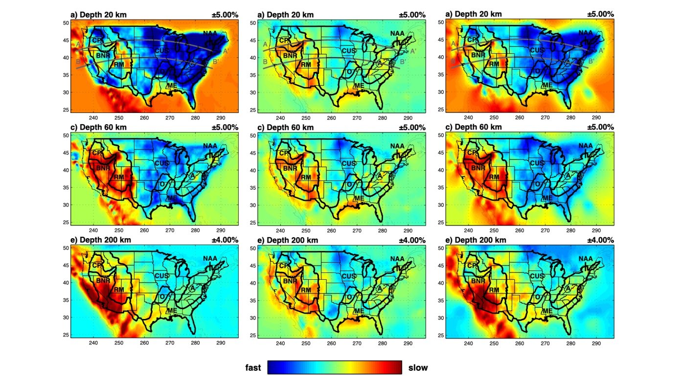
Slices through (left) Vp, (center), Vs, and (right) Vp/Vs ratio anomalies. Thick black lines denote various geologic areas.
What can we learn from looking at Vp/Vs? The pattern of variations is different from the Vp and Vs variations. At lithospheric depths, the lowest values of Vp/Vs are found in parts of the southwestern US, but also in the northeast and southern Canada. The highest values are seen in places like the Yellowstone region, and the eastern part of the Colorado Plateau. One thing that can contribute to high Vp/Vs is the existence of partial melt in the uppermost mantle. Other places in the central US, where no melt is expected, might have elevated Vp/Vs due to chemical differences. Future work will address the differing contributions of temperature and geochemistry on seismic velocity to better interpret lithospheric structure below the US.
Read more about this work in this article published in 2020.